Summarizing the log-cosh function is straight forward. However, let us dig deeper to find out what lies beneath the surface.
Simplicity wins: this especially holds true in data analytics, because throwing the most complex model at the data does not guaranty any success. The following writeup will establish basic terminology and build upon the said terminology towards the use of log-cosh function to illustrate clear purpose of the certain models and algorithms and how they work.
What is the loss function? Why do we need it? How do we use it?
In layman’s terms, data scientist running a neural network model can be described as an archer who first looks at the arrow, then at the target, and plunks the arrow towards the target.
Then the analysis begins: Has the arrow hit the bull’s eye? If not – how far is the arrow from the bull’s eye? What is the elevation of the arrow? How to account for archer’s paradox? Which begs a question, how does the archer correct the aim to account wind factors so next time we hit the bull’s eye and continue hitting it with each next arrow? How does the archer quantify his performance by measuring where the arrow lands on the target?
In supervised learning, the quantification of model’s performance is a measurement of the distance, as a mathematical difference, between the prediction and real-world measurements.
In analytics, the measurement how far is predicted value from the actual value could be done manually, which is literally completely unrealistic for any datasets; or, it can be done by utilizing computing power to compare the outcomes and measurements, which is computationally expensive and economically might not be feasible; or, it can be done by use mathematical functions.
Mathematical function is a process where an outcome, y, is defined as a function of variable x such as y = 2x+1-15; this contrasts with mathematical equation where we identify certain mathematical expression equates certain value such as 2x+1-15 = 0 or 2x+1 = 15. The critical distinction between the two notations, thus between function and equation, is in finding the outcome variable y for any given ever-changing variable x (as certain conditions are met) as opposed to finding a value of variable x for the equation given the same conditions.
Loss functions, also known as cost functions or objective functions, are mathematical functions which measure how close are models’ predictions to the real values targeted with ML model.
If the predicted value equals true value, then the loss function has the value zero; hence, we say the loss function is at its minimum. Thus, to minimize the loss function means to get prediction values as close to the true values as possible, which gets the loss function to its minimum.
Because neural network (NN) models are mathematical functions themselves – it is critical to delineate between inputs of neural network (NN) model and inputs of loss function (which are predictions) and establish the relationship between those two functions (by use of gradient descent).
NN model is comprised of one or multiple perceptron neurons where each perceptron is a linear function whose inputs are values of features of the dataset; while, the input values for loss function are the outputs of NN model (the predictions) and the real values from the dataset.
Perceptron, mathematically, is a linear function, often written up as f(x) = ax+b; where attribute b denotes the y intercept (bias) and attribute a identifies the slope of the said linear function. The perceptron takes as an input values x which are measurements of the feature, the importance of said feature expressed as weights as attribute a, and the bias which is either mathematically expressed as the y intercept (the inherit bias from the measurements) or modifiable backpropagated (beginning) value introduced to the model in the next iteration of the model. For perceptron with multiple features, has the output of as sum of the said features; thus, creating the perceptron’s mathematical function.
So, now we understand the inputs and outputs of the perceptron and what does loss function do for it.
So . . . how do we use it?
As noted above – the perceptron performs a linear regression and comes up with a function which will be used to provide future predictions, then the same function is used to produce prediction y’; the loss function takes y’ predictions as the input and measures how close the predictions are from true values, y (the dependent variable), and calculates attributes a and b, in other words: provides new bias and intercept. The objective of loss function is to find attributes a,b of linear function f(x) = ax + b which get predictions as close to the true value as possible. Then, Gradient Descent takes the loss function as its own input and through iterative process figures out how to minimize the loss function for attributes a and b for each tuple of data and find the fastest route to global or local minimum of the function.
So, it is obvious NN models are tuned by altering the multiplier weight (a) and bias (b) of individual input feature until predictions created by linear function are as close to original values as possible. The weights used for the next iteration of certain perceptron are calculated by loss function and sent back to the perceptron via gradient descent. This process is repeated until the loss function is minimized, meaning the predicted values are as close as possible to true values.
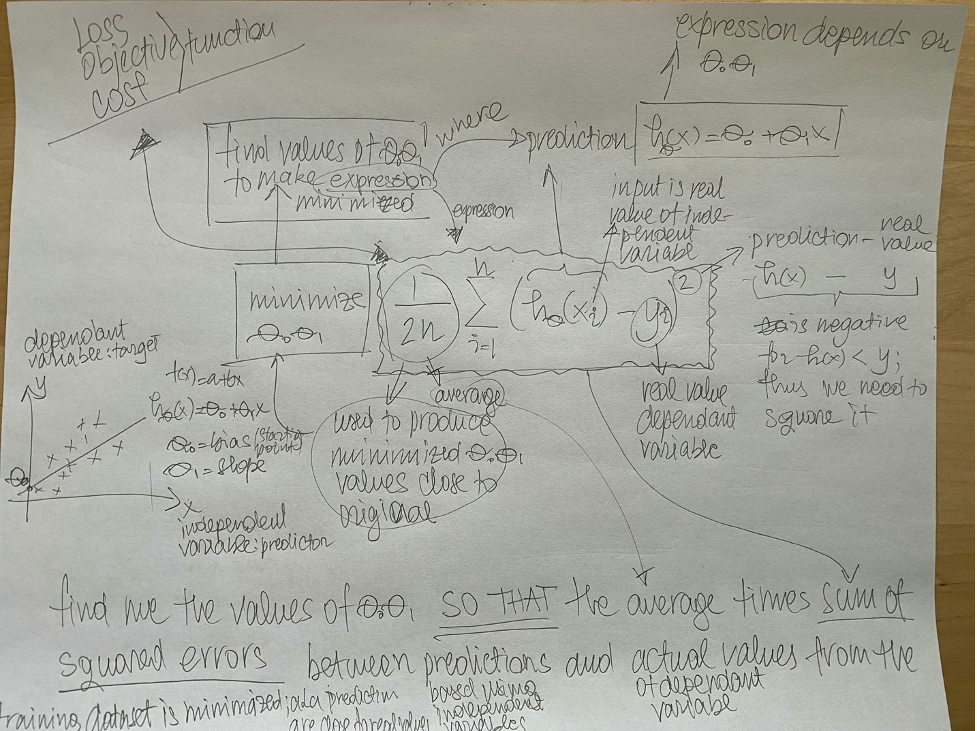
For our f(x) = ax + b linear function we can use the mean square error loss function as unpacked in the Figure 1.

How do we choose functions to measure the difference between predicted outcome and the true value?
It depends.
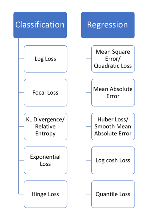
Loss functions are dependable on the type of analytics performed: classification or regression. In the Figure 2 one we see few main loss functions identified by the type of analytics.|

As seen in the Figure 2, there are variety of the loss functions. But, they do have several attributes in common. All of the function have to be differentiable; in other words, a derivative of said function has to exist for all the x values in the dataset. This is critical because, the second derivative of the loss function is the slope; and, calculating the slope is critical part of gradient descent. Thus, if a function is continuous, which is completely opposite from a differentiable function – then it cannot be used in the gradient descent.
The second derivative of loss function also acts as the multiplier of the “step” for gradient descent. As the 2nd derivative becomes smaller, so does the step taken by gradient descent towards the local/global minima. Which suggest, by changing the loss function, we directly change the step of gradient descent and control how the attributes a,b of f(x) response to the input values of x. This is probably the most critical piece of the whole process of choosing the loss function.
Another common attribute shared by all loss functions is ability to be used to calculate its global or local minima. For practical purposes, by finding the local/global minima is when the derivative of tangent line going through point x equals zero; thus, indicating the minima of the loss function, or in other words: at point x the prediction y’, which is generated by f(x) function produced by the linear regression, equals the true value (the dependent variable) from the dataset.
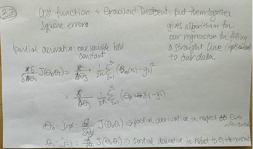
Yet another important attribute common to all loss functions is ability for loss function to accept the values for both attributes of f(x)=ax+b: a and b. This is critical part because the partial differentiation necessary to identify bias and the slope means: when we perform differentiation of attribute a, we hold attribute b as a constant and other way around, as seen in the Figure 3.

Which brings us to Logarithm of the hyperbolic cosine of the prediction error
(Log-Cosh) Loss Function . . .
Log-Cosh is quite similar to the mean square error loss function; “[it] works mostly like the mean squared error, but will not be so strongly affected by the occasional wildly incorrect prediction (Grover, 2018).”
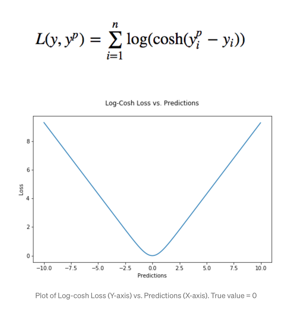
If we examine the graph in Figure 4, we can see the log-cosh being quadratic function – creates a parabola which is opened up; however, it has very evenly (linearly) distributed gradient until gets really close to the local minima; hence, not strongly affected by the incorrect predictions.


Best of luck!